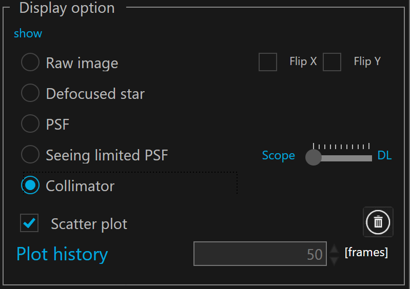
Display Collimator
To display the collimator tool (CT tool), you must set the display option on "Collimator". The CT tool is central to telescope collimation as it provides users with quantitative feedback for adjusting the collimation screws based on optical aberrations extracted from the wavefront. This section offers information on using the CT tool, along with advice and recommendations for proper telescope collimation. It also refers to tutorials and documents on the same topic. We strongly recommend that new SKW users thoroughly read this section and the related documentation before starting the collimation of their telescope.
The view port is empty if there is no defocused star analyzed.
The main goal of this view port is to provide a quantitative feedback during the alignment (collimation) process of your telescope throught a collimation (CT) tool..
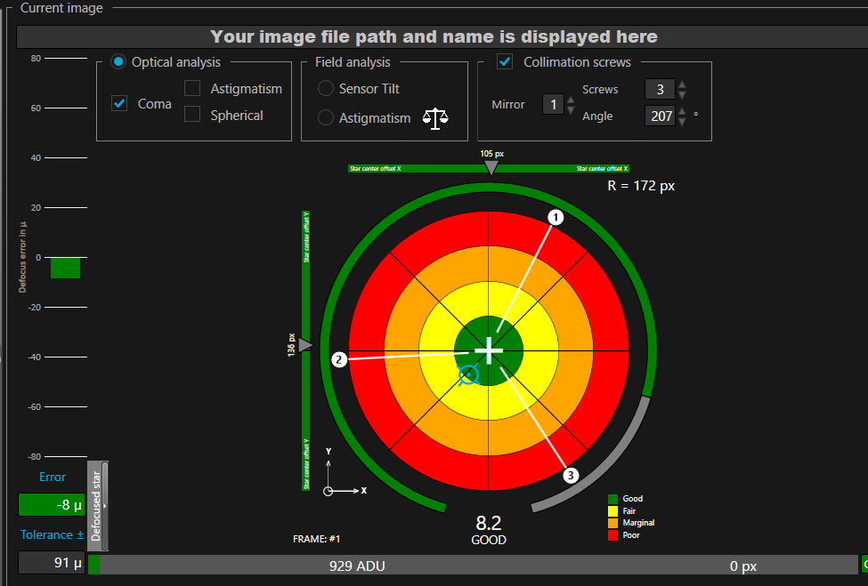
The file name of the currently loaded raw image is displayed on top.
The Collimation (CT) tool features a defocus error vertical gauge on the left. This gauge provides, in microns (metric), the signed difference between the expected defocus (calculated from the best focus point for the current telescope, wavelength in use, and selected SKW model) and the actual defocus measured by SKW.
This value is directly translated into focuser travel motion, assuming the use of an external focuser. A negative sign indicates the defocus is too small, while a positive sign indicates the defocus is too large. We recommend aiming for the smallest possible defocus error by fine-tuning the focuser based on the value reported by this gauge. Ideally, you should target a defocus error within one-third of the tolerance value if possible (displayed at the bottom of the gauge) or at least within the green zone.
Large defocus errors will eventually decrease collimation accuracy. If the defocus is achieved by moving one of the telescope mirrors rather than an external focuser, the defocus error provided is still useful for evaluating the optical defocus accuracy but not for adjusting the focuser, as optical magnification comes into play.
The best course of action is to first aim for a defocused star diameter in pixel as close as possible to the expected value provided by SKW in the input frame information. The sign indicates whether you are under- or over-defocused, see How to capture a suitable defocused star for further information.
The horizontal gauge below the CT tool target displays image intensity levels in ADU. If there is any saturation, the number of clipped pixels will be displayed on the left side of this gauge. Hot pixels are automatically removed by SKW processing, so this number only reflects image saturation.
For good SNR, aim for intensity values between half and two-thirds, below clipping, of the camera's ADU full scale. The stars used for SKW analysis must not be saturated.
 A red cross is displayed over the viewport when the star is saturated does not provide accurate wavefront.
The central target is used to display collimation information, scores, and other useful data. The goal is to bring the rotating blue cursor as close as possible to the center of the target, within the green zone.
The information displayed in and around the target depends on the analysis selected by the user, either the score for optical (aberration) analysis or image tilt and off-axis astigmatism for field analysis (note that more than one star is necessary for field analysis).
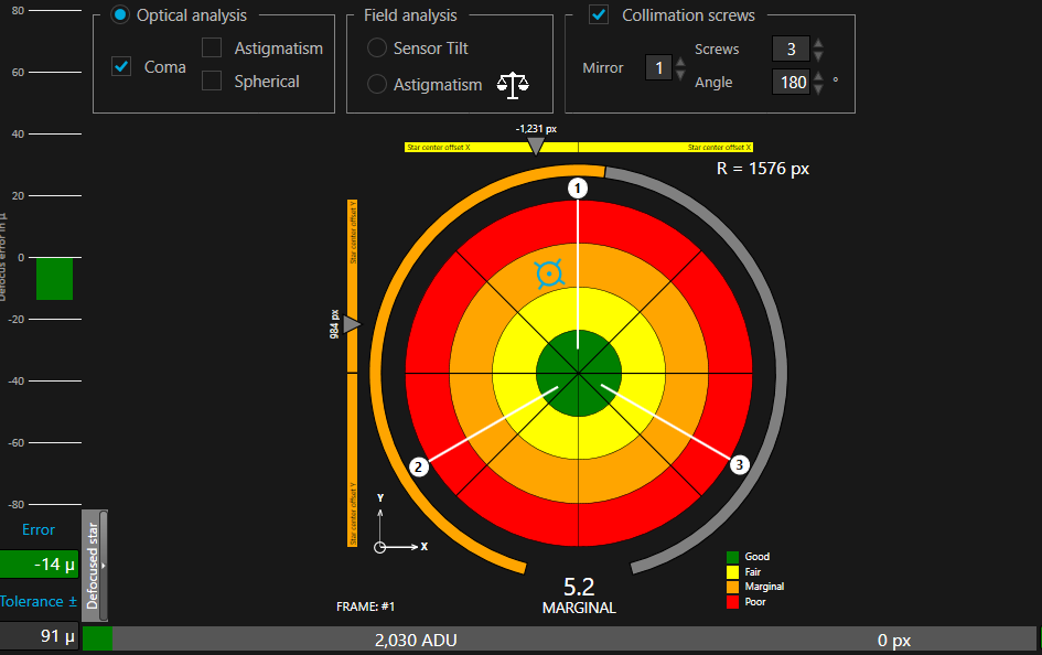
There are three panels at the top of the CT tool. The two on the left are used to select the type of analysis to perform, while the one on the right is used to position the collimation screws for both mirrors or the screws used to adjust a tilt/tip image train control mechanism. (for each configuration the user can select either 3 or 4 screws).
The 3 or 4 collimation screws (or tilt/tip image control adjustment screws) will be displayed once the "Collimation Screw" box is checked. The user can select how many screws are available (3 or 4) for a given configuration (mirror or image tilt/tip control mechanism) using the "Screws" field. They can also specify which mirror, when applicable, is considered for collimation using the "Mirror" field, and set the angular position of the screws (assumed to be equidistant from each other) using the "Angle" field.
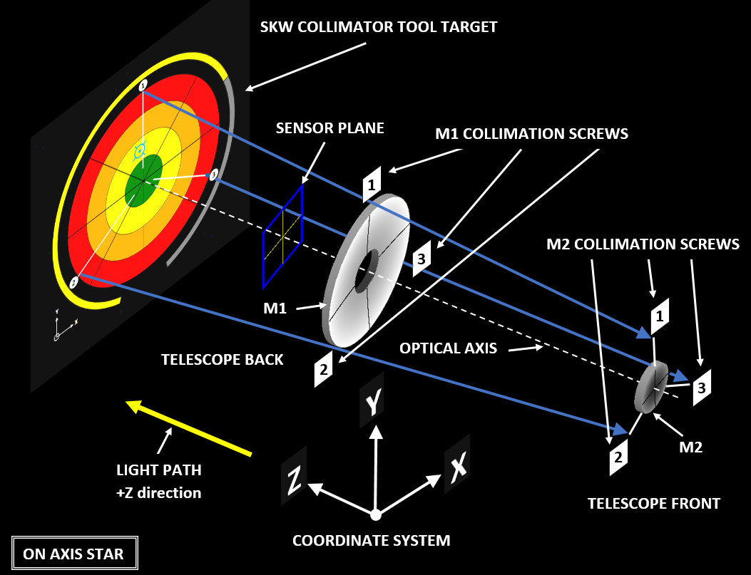
This visualization tool in the CT target is designed for user convenience and easier collimation. Users should label the screws 1 to 3 (or 4) and adjust the angular position for the selected screw set (mirror or image tilt/control) in the target by referencing the raw images. For example, placing a hand or an object near a screw to cast a shadow visible in the image can help identify the screw’s position. The target reference system is identical to the raw image displayed in SKW.
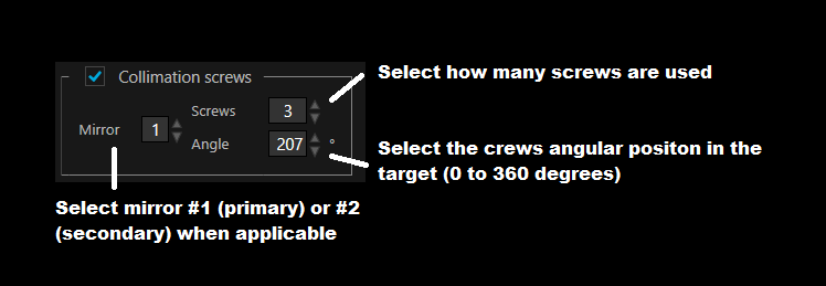
The angle of the collimation screws must be defined for each mirror or tilt/tip image control device.
To select the mirror, just select the mirror number. The number can be entered by pressing the key 1 or 2 or by acting on the spinner on the right side.
The angle can be adjusted by entering a value in degrees between -360 and +360 or by acting on the spinner on the right side.
Both angles are stored inside the selected instrument and save in the workspace.
Below is a figure describing how the CT tool aligns with the image captured by the telescope (assuming only three mirror collimation screws per mirror in this case). Here, it is assumed that the image captured by the user's acquisition software uses the same reference frame system as shown in the figure below.
The use of the X or Y flip checkboxes next to the SKW raw image viewport selection (in "Display Options") impacts the reference of the image and, therefore, the target and screw orientations, as SKW uses the same reference frame system for both. However, the image displayed in the user’s imaging acquisition software may have a different orientation. Using the tilt X and Y options in SKW allows the user to make both match for consistency and convenience.
Please refer to our tutrial for labling collimaiton screws for SKW:
XXXXXXXXXXXXXXXXXXXXXXXXXXXX
Blue dots scattered over the target represent the results of previous analyses, showing the trend of the collimation process. To view the score of each dot, hover over it with the mouse cursor to display the tooltip.
To disable the scatter plot, uncheck the "Scatter Plot" checkbox below.
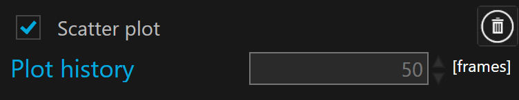
To clear the scatter plot, click on  button
To change the scatter plot history (the maximum number of blue dot visible on the target). By default 50, you must disconnect SKW change the value and connect.
OPTICAL ANLYSIS:
This panel, when checked, is dedicated to the analysis of aberrations (from the measured wavefront), including coma, astigmatism, and spherical aberration, which are all primary (basic) aberrations. The analysis is performed on the star displayed in the "Defocus Star" viewport (the selected star). Typically, this star should be placed at the center of the imaging camera sensor, which, by design, should be close to the telescope's optical axis when collimated.
The user can select any combination of the three basic aberrations; however, we recommend analyzing one aberration at a time.For spherical aberration, there is no angular information (dependency); therefore, the target is set as a simple circle filled with a solid colour corresponding to the score displayed below it. Spherical aberrations are usually related to the spacing between the mirrors or between the telescope (or camera) and the field lens (corrector). The rotating cursor on the target will be positioned based on the aberration level relative to the telescope's optical performance and the simulated seeing value FWHM (in arcseconds, ") selected by the user in the "Simulation" section at the bottom left of the SKW GUI. This value is used for calculations, such as scoring and PSF simulation.
Since the seeing conditions during collimation may differ (it may be worse) from those expected during normal telescope operation, this value can be adjusted independently of the "Local Seeing FWHM" value set in the instrument settings and displayed in the "Input Frame Information" section (on the right side of the SKW GUI).
Playing with optical analysis does not require a new frame analysis because all aberrations are calculated together in a single pass. The target is hidden when only the spherical aberration is selected. Since the spherical aberration is axisymmetric there is no directional information related to such aberration, unlike for coma or astigmatism.
The star center offset Y and X bars (top and left sid eof the target) shows the distance in pixels of the selected defocused star from the camera frame center.
A tooltip displays the values of each bar cursors (gray triangle). The defocus error tooltip shows also the defocus tolerance.
As collimation actions (tighten or releasing collimation knobs) slightly push the telescope out of the defocus tolerance and tranlate the image in the cmaera. After each move of the collimation knobs you must check the defocus error and if the bar become orange or red you must move the focuser in the opposite direction to restore the expected defocus. Most likely the star may need to be re-centered as well. Also the star may need to be recenter.
The distance R, in pixel, of the selected defocused star from the center of the image is displayed on the upper right corner in pixel.
The score of the selected optical analysis is displayed by a rotating cursor hovering over the target. You can also read the score below the target and check whether it is classified as poor, marginal, fair, or good.
The score ranges from 0 to 10, where 0 is the worst and 10 is the best. The goal is to achieve a score of 8 or above, which is in the green zone.
The score is calculated for the selected aberration only (coma, astigmatism, spherical, or any combination). It is computed relative to the "simulated" seeing value entered by the user, located at the bottom left of the SKW GUI under "Simulation."
Since most telescopes at most locations are seeing-limited (relative to the simulated seeing value provide by the user), achieving a score of 8 or higher indicates that the alignment of the telescope optics (collimation) is sufficiently precise for operational use of the scope under this seeing. Beyond this point, further collimation is certainly possible but it does not provide additional value, as it reaches the point of diminishing returns.
To help knowing which collimation screw must be tighten or loosen, SKW is able to superimpose the position of the three screws on top of the collimator target, as discussed above.
For most telescopes, especially those with a spherical mirror, either M1 (primary) or M2 (secondary), the optical axes of the telescope are superimposed (congruent) as long as there is no on-axis coma—typically at the centre of the camera sensor. This is all that is needed to collimate the telescope, aside from possible adjustments to the spacing between the mirrors or between the telescope’s visual back and the camera.
For most optical layouts, spherical aberration increases much more slowly than defocus. Sensitivity to mirror spacing is typically low, but this may not hold true for the field lens (corrector). Even a few millimetres of offset, either on the telescope or the camera side, can result in significant spherical aberration and potential vignetting at the field edges.
Using a plate-solving or equivalent tool to measure the telescope's focal length will likely yield a value that differs by a few percent from the nominal specification for the telescope. This is normal and expected. During production, there are always tolerances involved. Mirrors are typically paired to optimise optical performance, and the actual focal length is rarely identical to the nominal value. A small percentage difference is common, but for long focal lengths, this can appear substantial in absolute terms. For example, a 2% increase in a 2m focal length amounts to 40mm—just over 1.5 inches. While this might seem significant, it is entirely normal.
Telescope manufacturers typically adjust M1 to position the resulting focal plane (when collimated) at a specified back working distance (BWD). This distance is much more critical than the actual focal length, and users should place the camera at this location for optimal telescope performance, aiming for an in-focus image at the manufacturer-specified BWD.
The actual focal length is a poor proxy for mirror spacing. Adjusting the mirror spacing to match the nominal (specified) focal length is not recommended. The correct figure of merit is the level of spherical aberration. The actual focal length will almost always differ from the nominal value, and this is important to keep in mind.
For collimation, observe the angular position of the rotating target and adjust the collimation screws of the mirror located near or opposite the indicated direction. You may need to turn more than one screw. A screw location tool is helpful to identify which screws to act on. Since every telescope has a different mechanism for mirror adjustment, it’s impossible to specify whether you should turn the screws clockwise or counterclockwise, or by how much. You may need to experiment, but once you observe the effect (increase or decrease in the score), this knowledge will guide future adjustments for that specific telescope.
Typically, you should pull the mirror (either M1 or M2), assuming you are behind it, in the direction indicated by the target cursor. In telescopes with two aspherical (non-spherical) mirrors, like an RCT (Ritchey-Chrétien Telescope), coma correction must be performed using the appropriate mirror. Unless one of the mirrors (usually M2) has both translation (2 degrees) and tilt (2 degrees) adjustment capabilities, alignment of the mirror axes can only be achieved iteratively by adjusting the tilt and tip of both mirrors. In such cases, it is strongly recommended to use M1 to correct on-axis coma and M2 to balance off-axis astigmatism. This is particularly critical for an RCT. Adjusting the wrong mirror leads to divergent and unstable collimation. This is a common mistake when collimating an RCT, as in most other telescopes, M2 is used for coma correction and collimation. However, for an RCT (or similar telescopes), M1 should be used for coma correction, while M2 is reserved for astigmatism adjustment.
As an example the screenshot below shows that to correct coma for this scope (based on the location of the collimation screws relative to the camera and image, as labelled by the user), you should adjust screw #1, the one closest to the rotating cursor, until the scope is in the green zone. It usually takes a few iterations and small corrections to achieve this goal. Having access to the score value and the location of the correction relative to the screws provides an effective, quantitative method to achieve optical collimation. The process would be similar for astigmatism. For spherical aberration, however, there is no angular information since it is an axisymmetric aberration; only the score and its sign are relevant.
Aside from optical spacing, when the scope is out of collimation—meaning the mirror axes are not congruent—the resulting focal plane is somewhat tilted relative to the focal plane when the scope is properly collimated. This results in a gradient of defocus across the image (manifested as variations in star FWHM or HFD), which is normal. It does not necessarily indicate that the sensor itself is tilted relative to the optical axis of the collimated scope; it may or may not be.
Therefore, the proper course of action is to first collimate the scope by correcting coma and astigmatism. Only after that should any sensor/image tilt adjustment mechanisms be used, if residual tilt remains. By observing star sizes (e.g., FWHM), one cannot distinguish whether the tilt (gradient of defocus) is due to a collimation issue or sensor tilt. Proper optical aberrations must be used for alignment.
Once collimated, the FWHM values should either be identical across the entire field or axisymmetric (balanced) relative to the sensor’s centre. When this is not the case, FWHM values are ambiguous and cannot provide effective collimation information. We strongly advise against adjusting any sensor/image tilt controls until the scope has been optically collimated first.
To learn more about alignment procedure refer to our documentation and tutorial:
Telescope with at least one spherical mirror (SCT, CDK, iDK, ...)
https://www.innovationsforesight.com/Wavefront/SKW_Scope_with_Spherical_Mirror_Alignment_011522.pdf
Telescope with both aspherical mirrors (RCT, ...)
https://www.innovationsforesight.com/Wavefront/SKW_RCT_Alignment_011522.pdf
FIELD ANLYSIS:
The SKW CT tool features two additional analyses using multiple stars, typically from an actual star field or an image created by superimposing the same defocused star at different locations. In both cases, it is important to spread the stars across the field for uniform coverage, as this improves the quality of the analysis. SKW will automatically search for and select usable stars based on the star quality filter parameters set by the user., see Load, Locate, Select and Analyze selected star .
Sensor Tilt uses the defocus aberration (defocus is an aberration like any other) gradient across the field to compute image tilt. It processes a star field assuming that any defocus gradient is a combination of field curvature (if present) and mechanical image tilt. It is crucial to collimate the telescope FIRST before using this tool, as a misaligned telescope results in a tilted focal plane. Defocus aberration is different from FWHM or HFD, as it only measures the optical defocus level. In contrast, FWHM and HFD combine the effects of all aberrations, including spherical aberrations, leading to ambiguity. For example, it is impossible to separate an FWHM gradient caused by sensor/image tilt from one caused by collimation errors. SKW uses different aberrations for different tasks, and in this context, defocus is the correct figure of merit for measuring sensor/image tilt. The CT tool provides users with quantitative information about tilt (even in the presence of field curvature) in relation to the tilt/tip adjustment screws defined by the user. The process is essentially the same as collimation (optical analysis) in terms of screw labelling and adjustment.
The screenshot below shows a typical result for a star field (27 stars were selected by SKW in this example). In this configuration, we assumed that the tilt/tip mechanical corrector device, placed somewhere in the optical path behind the telescope's visual back, features four screws (SKW can also be configured for three screws). These screws, once again, have been labelled and positioned within the TC tool by the user in the same way as for telescope collimation when performing optical analysis.
 When either tilt or balanced astigmatism, is selected in the "field analysis", the "optical analysis" settings selections do not apply.
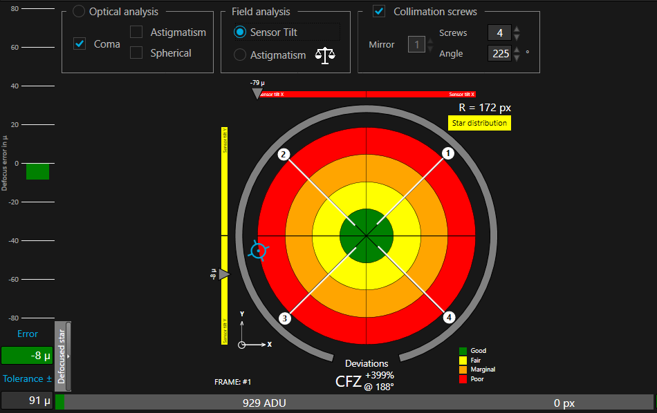
The tilt is reported in several ways. The primary information is conveyed by the rotating cursor, which indicates the level (relative tot the CFZ) and direction of the tilt inside the target. In this case, the score below the target has been replaced by the maximum deviation in the image frame from the critical focus zone (CFZ) at the worst position, which is located somewhere at the edge of the field (sensor). A value of 100% means that, at this worst location, the image tilt induces a defocus equal to the CFZ (the CFZ is calculated based on the telescope's optics and the wavelength selected by the user in SKW). At a minimum, we want the worst deviation to be no greater than one CFZ, i.e., at or below 100%. However, it is recommended to reduce the tilt further until the cursor is within the green zone using the collmation screws, in this case above we would adjust screws 2 and 3, or 1 and 4. The smaller the better.
At the top and left of the target, two gauges display the deviation in microns (metric) at the edge of the image (sensor), including the sign. Finally, on the upper right of the target, there is a flag labelled "Star distribution." If it is red, this indicates that there are either not enough stars for the calculation or that they are poorly distributed across the field, leading to a bad conditioned numerical solution.
As with the "optical analysis," the screws and the X and Y reference axes used by the target are related to the image provided to SKW. If there are inversions in either axis, you can use the "Flip X" and "Flip Y" checkboxes available in SKW next to the raw image viewport selection.
Balancing Astigmatism is typically used with telescopes that have two aspherical mirrors, such as Ritchey-Chrétien Telescopes (RCTs). In such systems, canceling on-axis coma alone is not sufficient for collimation. The telescope cannot be aligned using only a single on-axis star. Instead, it is necessary to use off-axis astigmatism observed in off-axis stars. In this case, it is not so much the amplitude of the astigmatism but its axial symmetry relative to the center of the sensor (assumed to be coincidental with the optical axis when collimated) that is critical. This symmetry ensures proper alignment of the telescope to its optical axis by making both mirror axes congruent..
All optical systems exhibit off-axis aberrations, typically coma and astigmatism, which increase with radial distance from the optical axis of the system:
- Coma increases linearly with the radial distance (linear with field angle).
- Astigmatism increases the square of the radial distance (square with field angle).
Optical designs are optimized to minimize these off-axis aberrations within a defined corrected circle. This corrected circle represents the largest field of view (field angle) where the image quality remains operationally good, often defined by a Strehl ratio (SR) of 0.8 (80%) or higher, which indicates diffraction-limited performance by definition.
It should be noted that a well-collimated optical system does not exhibit on-axis coma or on-axis astigmatism; these are strictly off-axis aberrations. Spherical aberration, on the other hand, may be present due to spacing errors. Unlike coma and astigmatism, spherical aberration is generally uniform across the field and does not depend on the field angle.
Below is an example of unbalanced off-axis astigmatism. At a given radius (or distance, corresponding to a field angle) from the optical axis—practically, near the center of the sensor or a nearby reference point where there is no coma or astigmatism if the telescope’s optical axis is correctly aligned with the sensor—one observes that the astigmatism is not symmetric (unbalanced). Both the magnitude and the axial direction of the astigmatism are asymmetrical, indicating misscollimation.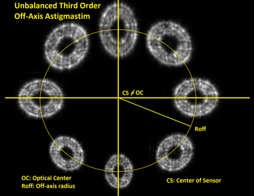
What we are loking for is shown below. Wither a tnaential or radial near cosntant magnitude asigmastim at some distance (field angle) off-axis. Those are two example of balacned astigamstim, the goal.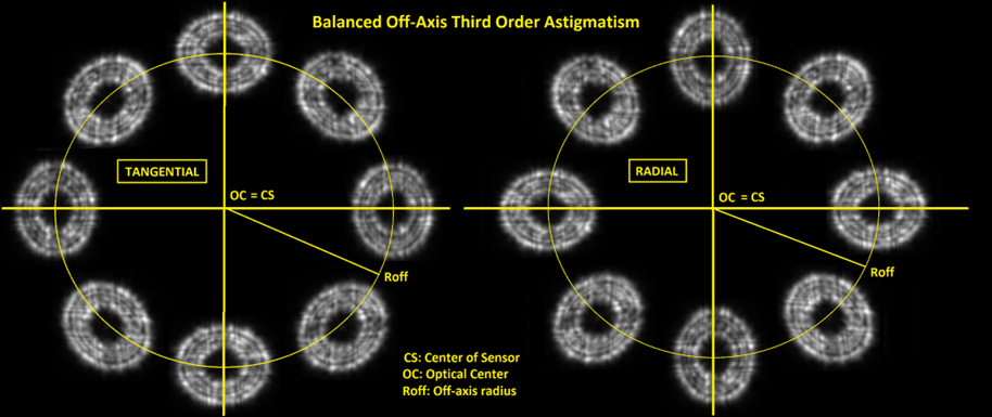
What we are aiming for is illustrated below: either tangential or radial astigmatism with nearly constant magnitude at a certain distance (field angle) off-axis. These are two examples of balanced astigmatism, which represent the desired outcome.
The SKW CT tool measures the level of balanced astigmatism using a single numerical value for convenience. To achieve this, as with the image/sensor tilt discussed earlier, several defocused stars across the field are required. This can be done using either a well-distributed star field or a set of defocused stars placed at a nearly constant distance from the center of the sensor.
The figure of merit is the relative value of unbalanced astigmatism, expressed as a percentage, the smaller the better. A rotating cursor in the target is placed at the location where the maximum unbalanced astigmatism is detected, providing guidance for adjusting the proper collimation screw of the secondary mirror (usually M2).
Below is an example showing strong unbalanced astigmatism, here 87%, located at 45 degrees in the direction of the upper-right corner of the sensor. Corrective action can be performed by adjusting screw 2 and/or screw 3. The magnitude and direction of the correction (clockwise or counterclockwise) depend on the mechanical design of the telescope.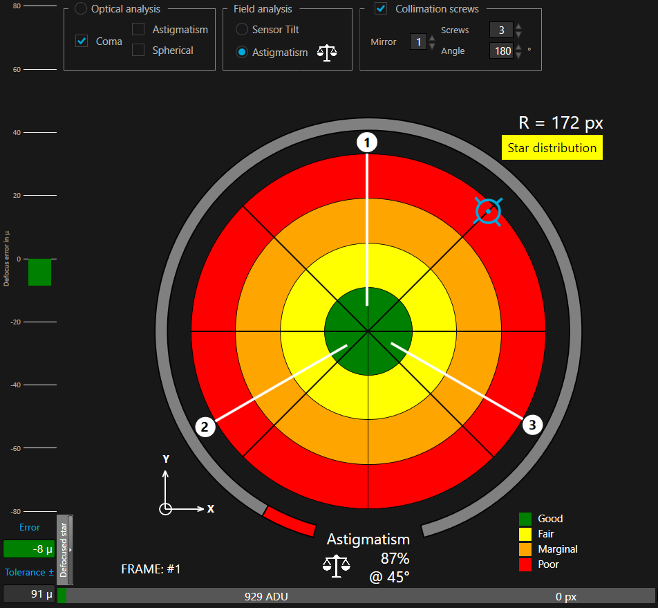
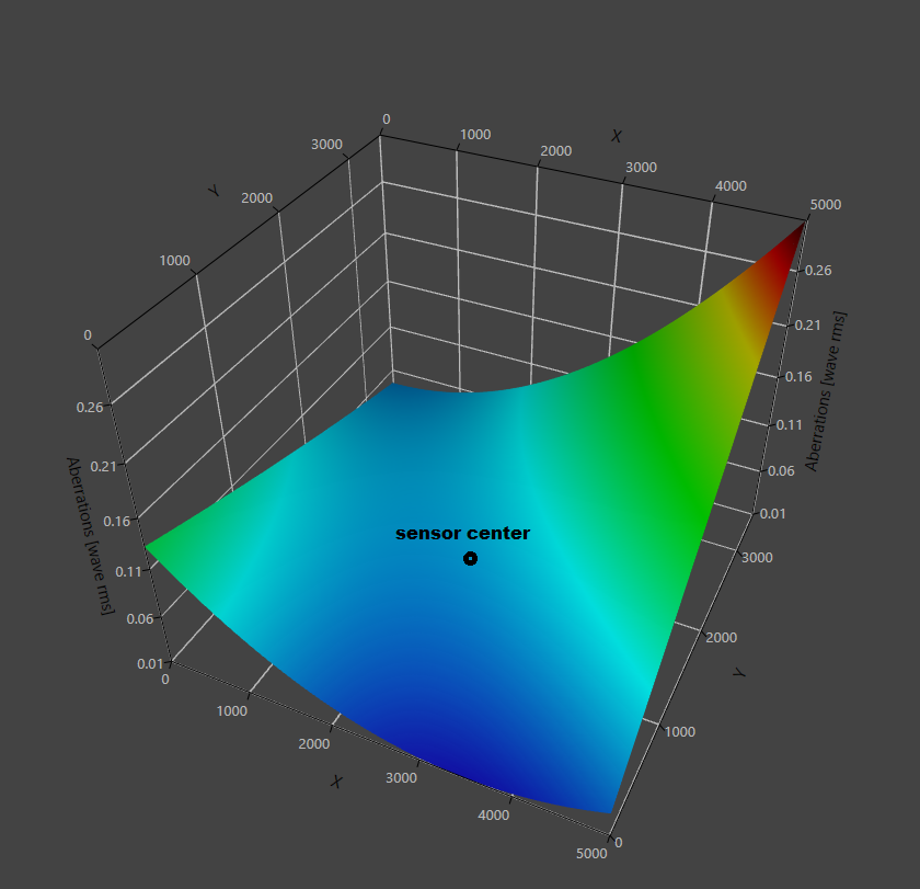
The SKW Pro version provides field-dependent aberration analysis. By selecting both oblique and vertical astigmatism Zernike annular polynomials, a 3D plot of astigmatism magnitude across the field can be generated. In this plot, the center of the sensor corresponds to the middle of the graph, representing the on-axis point.
This visualization clearly highlights that the total astigmatism magnitude is not axisymmetric, with larger values occurring towards the upper-right corner of the field (at 45 degrees), as noted by the CT tool above.
Notice: SKW Pro is the professional version of SKW, offering comprehensive optical analysis, including Zernike coefficients, wavefront data, field-dependent MTF data, and more. It is available through an annual subscription. For a quote, please contact Innovations Foresight directly. Bothe SKW CT and Pro use the same engine our AI4Wave wavefront sensing technology.